Chapter 8Training a Model: Loss, Gradients, and Backpropagation

The Question: How Does a Network Get Good?

A freshly built network has random weights, so its predictions are random too. Training is the process of nudging those weights, over and over, until the predictions become accurate. To do that automatically, we need to answer three questions in turn: How wrong are we right now? Which direction makes us less wrong? And how big a step should we take? Each question has a clean answer, and together they form the training loop.

Step 1: Measuring How Wrong We Are (Loss)

Before a model can improve, it needs a single number that says how badly it is doing. That number is called the loss (or error), and the rule is simple: lower is better. A loss of zero would mean perfect predictions. The function that computes it is the loss function.

A common one for predicting numbers is mean squared error: for each example, take the difference between the prediction and the correct answer, square it (so that being wrong in either direction counts as positive, and big mistakes count much more than small ones), and average over all examples.

def mean_squared_error(predictions, targets):
    total = 0
    for p, t in zip(predictions, targets):
        total += (p - t) ** 2     # square the gap
    return total / len(predictions)

print(mean_squared_error([3, 5, 2], [2, 5, 4]))   # (1 + 0 + 4) / 3 = 1.67

Now we have turned "how good is this model?" into one honest number we can try to shrink. Everything that follows is about shrinking it.

Step 2: Which Way to Adjust (Gradients)

We have a loss; now we need to know how to reduce it. Recall the foggy hillside from Chapter 5: you cannot see the whole landscape, but you can feel which way the ground slopes and step downhill. The loss is the height of that landscape, and our position is set by the model's weights.

The gradient is the "which way is downhill" information, computed for every single weight at once. For each weight it answers: if I nudge you up a little, does the loss go up or down, and by how much? Armed with that, we know precisely which direction to move each weight to make the model less wrong.

Step 3: Take a Small Step (Gradient Descent)

Knowing the downhill direction, we adjust each weight a small amount in that direction. Repeating this — step after step — is gradient descent. The size of each step is set by a number called the learning rate, and choosing it well matters more than beginners expect.

• Too large a learning rate and you leap right over the valley, bouncing wildly or even climbing — like taking giant strides down a hill and overshooting the bottom every time.
• Too small a learning rate and you inch along so slowly that training takes forever to make progress.
• A well-chosen learning rate descends briskly but safely toward the lowest point.

Backpropagation: Sharing the Blame

One question remains: in a deep network with many layers, how do we figure out each weight's gradient — its share of responsibility for the error? The answer is an algorithm called backpropagation, and its intuition is a team post-mortem after a mistake.

When something goes wrong, a good team traces the error backward: the final output was off, which means the last layer contributed in a certain way, which means the layer before it contributed in turn, and so on back to the start. Backpropagation does exactly this — it starts from the loss at the output and works backward through the network, assigning each weight its fair share of the blame for the error. That share is its gradient. The name is just "propagating the error backward."

The Training Loop

Now we assemble the four ideas into the loop that trains every neural network in existence:

1. Forward pass — feed an example through the network to get a prediction.
2. Compute the loss — measure how far the prediction is from the correct answer.
3. Backward pass — use backpropagation to find each weight's gradient.
4. Update — nudge every weight a small step downhill, scaled by the learning rate.

Repeat this for many examples, and then repeat the whole sweep through the data many times. Each full pass over the training data is called an epoch. With each epoch, the loss creeps lower and the model gets better.

Watching a Tiny Model Learn

Let us see it actually happen. The smallest meaningful example is learning a single weight w so that w * x matches a target. Our data secretly follows the rule "target is two times x," but the model does not know that — it starts with a wrong guess and must learn w = 2 on its own.

data = [(1, 2), (2, 4), (3, 6)]   # (x, target); the hidden rule is target = 2*x
w = 0.0                            # start with a wrong guess
learning_rate = 0.01

for epoch in range(100):
    for x, target in data:
        prediction = w * x
        error = prediction - target
        gradient = 2 * error * x          # how the loss changes with w
        w = w - learning_rate * gradient  # step downhill

print(round(w, 3))    # ends up very close to 2.0

Read what happens inside the loop. The model predicts, sees how far off it is, computes the direction that reduces the error, and nudges w that way — then does it again, hundreds of times, until w settles near 2. That is the entire essence of training, stripped to its bones. Real networks have millions of weights instead of one, but the loop is identical.

Watching the Loss Come Down

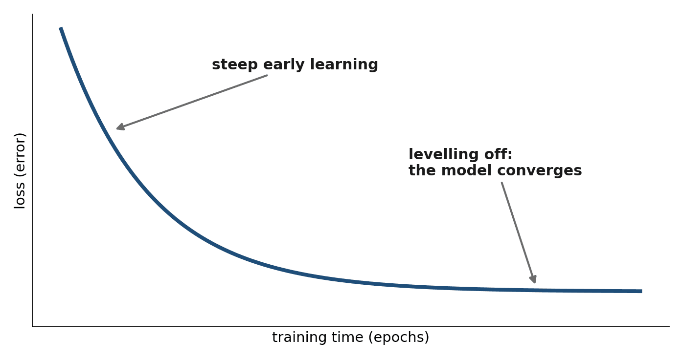
The clearest sign that training is working is the loss curve — a graph of the loss over time. A healthy curve falls quickly at first, then flattens as the model approaches the best it can do. If you ever train a model, watching this curve is your single best diagnostic.

When Training Goes Wrong

Three failure patterns are worth recognizing now, since you will meet them again when you fine-tune real models in Part V.

• The loss bounces or explodes — usually the learning rate is too high; the model keeps overshooting. Lower it.
• The loss barely moves — often the learning rate is too low, or the model is too simple (underfitting, from Chapter 6).
• Training loss keeps dropping but the model fails on new data — the model is overfitting, memorizing the training set instead of learning the pattern. This is why we always watch performance on held-out test data, not just the training loss.

Summary

Training turns a random network into a skilled one through a simple loop. A loss function condenses "how wrong are we?" into one number to minimize. Gradients tell us which way to adjust every weight to reduce that number, and gradient descent takes small downhill steps, sized by the learning rate. Backpropagation is how those gradients are computed across a deep network — by passing the error backward and assigning each weight its share of the blame. Repeat the forward pass, loss, backward pass, and update over many epochs, and the loss falls as the model learns. Watch held-out data, not just training loss, so you measure real learning rather than memorization.

We now understand how models learn in general. Chapter 9 applies all of this to a specific, foundational task — turning words into meaningful numbers called embeddings — which directly powers the search, memory, and retrieval your agents will rely on.